weekly_prices = [3.05, 3.04, 3.11]4 Array computations
In the previous chapter we stored data in plain Python lists, and we used the statistics module (and considerable manual work) to summarize it. That approach worked, but it was tedious. To do almost anything to every value in a list (add a tax to every price, convert every value to different units, or just add two lists of numbers together), we had to handle the values one at a time.
In this chapter we introduce NumPy (short for “Numerical Python”), the standard Python library for working with numerical data. NumPy gives us a new kind of container called an array, which makes numerical computations shorter to write and faster to run compared to using lists. Arrays are the foundation that nearly every other data science tool in Python, including the Pandas package we’ll use later, is built on top of.
By the end of this chapter you’ll be able to load numerical data into arrays, transform and summarize that data in a single step, filter it down to the values you care about, and even treat images as arrays of numbers.
4.1 Why arrays instead of lists?
To see some of the shortcomings of using lists for data processing, suppose we have the price of a gallon of gas (in dollars) for three weeks, stored in a list:
Now imagine the government adds a 100% tax, doubling the price of every gallon. If we wanted the new price for each week, it would be natural to try multiplying the list by 2, but lists don’t behave the way we might hope:
# Multiplying a list by 2 repeats the list instead of doubling each value
weekly_prices * 2
[3.05, 3.04, 3.11, 3.05, 3.04, 3.11]As you can see, that doesn’t double each price. Instead, multiplying a list by a number just repeats the list. And if we wanted to add a constant to each item, writing weekly_prices + 2 would produce an error rather than the new prices. To actually double each price we would have to reach into the list and update each value individually:
# Doubling each price, one value at a time
[weekly_prices[0] * 2, weekly_prices[1] * 2, weekly_prices[2] * 2]
[6.1, 6.08, 6.22]This works for three prices, but it would be impractical for a larger dataset.
Note
Python does have a tool for repeating an action many times without writing it out by hand: the loop, which we cover later in Chapter 8. But for the whole-dataset calculations that are common in data science, the array approach shown in this chapter is usually shorter and easier to read, so we will favor it throughout the book.
NumPy lets us express the same computation in one line. First, import the library (by near-universal convention, NumPy is imported under the short name np):
import numpy as npNow we can turn our list into a NumPy array with np.array() and multiply by 2:
price_array = np.array([3.05, 3.04, 3.11])

# Doubling the gas prices
price_array * 2
array([6.1 , 6.08, 6.22])The operation was applied to every element automatically. This idea, applying an operation to every element of an array at once, is called vectorization, and it is what makes NumPy so useful. Compared to lists, arrays give us two main advantages:
- Ease of expression. Element-wise arithmetic like
price_array * 2andprice_array + 2lets us say what we mean in a single short expression. - Speed. NumPy performs these operations in fast, pre-compiled code and stores values more compactly than a list, so computations on large arrays run faster and use less memory.
TipExercise
Here are three more weekly gas prices stored in a list: [3.20, 3.15, 3.18]. Turn this list into a NumPy array, then use a single expression (no loop) to calculate the prices with a three-dollar surcharge added to each (i.e., each price becomes 3 dollars higher).
NoteSolution
more_prices = np.array([3.20, 3.15, 3.18])

# Adding 3 dollars to every price at once
more_prices + 3
array([6.2 , 6.15, 6.18])4.2 An example dataset: a year of U.S. gas prices
To explore NumPy we’ll look at the price of gasoline in the United States over the course of a year. Gas prices change every week, so the data gives us a natural sequence to explore: how prices moved, how much they varied, and what fraction of weeks fell below a given threshold.
Our data comes from FRED (Federal Reserve Economic Data), a large public database of economic time series maintained by the Federal Reserve Bank of St. Louis. We’ll store the U.S. average weekly retail price of regular gasoline for 2025 in two NumPy arrays: gas_prices, which holds the price for each week, and gas_dates, which holds the corresponding date. Run the cell below to load the data; as with the data-loading code in the previous chapter, you don’t need to understand its details yet.
import pandas as pd

# Try to download the data live from FRED; if that fails (for example, when there
# is no internet connection), fall back to a saved snapshot of the same year.
try:
    from pandas_datareader.fred import FredReader
    gas_data_all = FredReader("GASREGW", start="2024-06-01", end="2026-01-15").read().reset_index()
    gas_year = gas_data_all[(gas_data_all["DATE"] >= "2025-01-01") & (gas_data_all["DATE"] < "2026-01-01")]
except Exception:
    gas_year = pd.read_csv("data/gas_prices_GASREGW_2025.csv", parse_dates=["DATE"])

# Pull the prices and dates out of the data table as NumPy arrays
gas_prices = gas_year["GASREGW"].values
gas_dates = gas_year["DATE"].values
Let’s take a look at the prices:
gas_pricesarray([3.047, 3.043, 3.109, 3.103, 3.082, 3.128, 3.148, 3.125, 3.078,
3.069, 3.058, 3.115, 3.162, 3.243, 3.168, 3.141, 3.133, 3.147,
3.12 , 3.173, 3.16 , 3.127, 3.108, 3.139, 3.213, 3.164, 3.125,
3.13 , 3.121, 3.123, 3.14 , 3.118, 3.125, 3.147, 3.177, 3.192,
3.168, 3.173, 3.118, 3.124, 3.061, 3.019, 3.035, 3.019, 3.056,
3.062, 3.061, 2.985, 2.94 , 2.895, 2.841, 2.811])This is an array of 52 numbers, one price per week. The first value, about $3.05, is the price in the first week of January. The matching gas_dates array holds the date of each week’s price, stored as NumPy datetime values:
# The dates of the first three weekly prices
gas_dates[0:3]
array(['2025-01-06T00:00:00.000000', '2025-01-13T00:00:00.000000',
'2025-01-20T00:00:00.000000'], dtype='datetime64[us]')Before computing any statistics, we can see the whole year at a glance using the Matplotlib skills from the previous chapter:
import matplotlib.pyplot as plt

plt.plot(gas_dates, gas_prices, '.-')  # '.-' draws dots at each data point connected by lines
plt.xlabel("Date")
plt.ylabel("Price per gallon ($)")
plt.title("U.S. weekly regular gas price, 2025")
plt.xticks(rotation=45)
plt.show()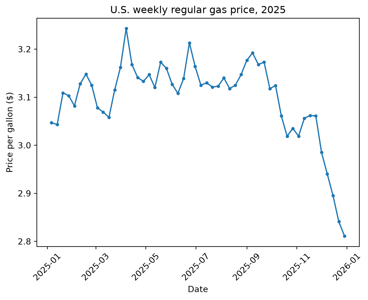
Prices rose through the spring, peaked in April, and drifted lower through the second half of the year, reaching their lowest point in late December. Throughout the chapter we’ll use these two arrays, and NumPy, to ask more precise questions about this story.
4.3 Creating arrays and their basic properties
We’ve already seen the most common way to make an array: pass a list to np.array(). For example, we can pass the list [10, 20, 30, 40] to the np.array() function to create an array of 4 elements:
example_array = np.array([10, 20, 30, 40])
example_array
array([10, 20, 30, 40])An important property of NumPy arrays is that all elements must have the same data type. For example, an array can hold all numbers or all Booleans, but unlike a list it cannot mix types.
To see what type of element is being stored in an array, we can access the array’s dtype attribute:
# The data type of the elements (float64 means decimal numbers)
gas_prices.dtypedtype('float64')Note that we write .dtype without parentheses, because it is an attribute of the array (a stored property) rather than a function we call.
What happens if you break the same-type rule and pass np.array() a list with mixed types? NumPy does not report an error. Instead it silently converts every value to a common type, usually strings:
np.array([1, "two", True])array(['1', 'two', 'True'], dtype='<U21')The quotes around each value show that everything, including the number and the Boolean, has become a string. Arithmetic will no longer work on this array, so an accidental string in a list of numbers is worth watching out for.
Similarly, we can see how an array’s elements are arranged using the shape attribute:
# The shape of the array: 52 weeks of prices in a single dimension
gas_prices.shape(52,)The .shape is reported as (52,), which tells us the array has 52 elements arranged in a single dimension. The trailing comma is Python’s notation for a one-element tuple (a parentheses-wrapped sequence of values); a 2D array would show two numbers here, like (4, 5). Two more useful attributes are .size (the total number of elements) and .ndim (the number of dimensions):
[gas_prices.size, gas_prices.ndim][52, 1]Sometimes we want to change the data type of an array, for example to view our prices as whole numbers of dollars. The .astype() method makes a new array with a different type:
# Convert the decimal prices to integers (the decimal part is dropped, not rounded)
gas_prices.astype(int)
array([3, 3, 3, 3, 3, 3, 3, 3, 3, 3, 3, 3, 3, 3, 3, 3, 3, 3, 3, 3, 3, 3,
3, 3, 3, 3, 3, 3, 3, 3, 3, 3, 3, 3, 3, 3, 3, 3, 3, 3, 3, 3, 3, 3,
3, 3, 3, 2, 2, 2, 2, 2])Finally, NumPy can generate arrays for us without starting from a list. np.arange() allows us to create an array of sequential integers, and np.linspace() produces a given number of evenly spaced values between two endpoints:
# Whole numbers from 0 up to (but not including) 10
np.arange(10)
array([0, 1, 2, 3, 4, 5, 6, 7, 8, 9])np.arange() can also take a start and a stop value. Like slicing, the stop value is excluded:
# Whole numbers from 1 up to (but not including) 11
np.arange(1, 11)
array([ 1, 2, 3, 4, 5, 6, 7, 8, 9, 10])# Five evenly spaced values from 0 to 1
np.linspace(0, 1, 5)array([0. , 0.25, 0.5 , 0.75, 1. ])
TipExercise
Use np.arange() to create an array containing the whole numbers from 5 to 15 (including both endpoints). Then use .astype() to make a version of that array whose values are floating-point numbers, and check its .dtype to confirm the conversion worked.
NoteSolution
# The stop value is excluded, so we use 16 to include 15
nums = np.arange(5, 16)
nums_float = nums.astype(float)

[nums_float, nums_float.dtype]
[array([ 5., 6., 7., 8., 9., 10., 11., 12., 13., 14., 15.]),
dtype('float64')]4.4 Indexing and slicing
Indexing and slicing arrays work just like they did for lists in the Python basics chapter. We use square brackets with a position (starting from 0), and we can use negative positions to count from the end:
# The price in the first week of the year
gas_prices[0]np.float64(3.047)# The price in the last week of the year
gas_prices[-1]np.float64(2.811)We can also take a slice to get a range of values. Here are the prices for the first five weeks:
gas_prices[0:5]array([3.047, 3.043, 3.109, 3.103, 3.082])Right away we can see that gas started the year a little over $3.00 a gallon. To say more, we’ll want to summarize all 52 weeks at once.
TipExercise
Use slicing to select and display the gas prices for the last five weeks of the year. (Hint: negative positions count from the end of the array.)
NoteSolution
gas_prices[-5:]array([2.985, 2.94 , 2.895, 2.841, 2.811])4.5 NumPy functions for summarizing and transforming arrays
This is where arrays are most useful. NumPy provides a large collection of functions that operate on an entire array at once, letting us answer questions about our data with a single line of code. These fall into two families.
The first family transforms every value: arithmetic like gas_prices * 147 applies the operation to each element. The second family reduces an array to a summary: np.mean(), np.median(), np.min(), np.max(), np.sum(), np.std(), and np.percentile() each collapse the whole array down to one number. You saw the statistics module handle some of these in the previous chapter; NumPy’s versions work directly on arrays and are much faster on large datasets.
4.5.1 Transforming every value at once
We saw earlier that we can do arithmetic on an entire array. Because each operation applies to every element, we can answer “what if” questions in a single line. For example, one U.S. dollar was worth roughly 147 Japanese yen during this period. So what was each week’s gas price in yen?
# Convert every weekly price from dollars to yen
gas_prices * 147
array([447.909, 447.321, 457.023, 456.141, 453.054, 459.816, 462.756,
459.375, 452.466, 451.143, 449.526, 457.905, 464.814, 476.721,
465.696, 461.727, 460.551, 462.609, 458.64 , 466.431, 464.52 ,
459.669, 456.876, 461.433, 472.311, 465.108, 459.375, 460.11 ,
458.787, 459.081, 461.58 , 458.346, 459.375, 462.609, 467.019,
469.224, 465.696, 466.431, 458.346, 459.228, 449.967, 443.793,
446.145, 443.793, 449.232, 450.114, 449.967, 438.795, 432.18 ,
425.565, 417.627, 413.217])Or, returning to our tax example, what would each price be with a $2-per-gallon tax added?
gas_prices + 2array([5.047, 5.043, 5.109, 5.103, 5.082, 5.128, 5.148, 5.125, 5.078,
5.069, 5.058, 5.115, 5.162, 5.243, 5.168, 5.141, 5.133, 5.147,
5.12 , 5.173, 5.16 , 5.127, 5.108, 5.139, 5.213, 5.164, 5.125,
5.13 , 5.121, 5.123, 5.14 , 5.118, 5.125, 5.147, 5.177, 5.192,
5.168, 5.173, 5.118, 5.124, 5.061, 5.019, 5.035, 5.019, 5.056,
5.062, 5.061, 4.985, 4.94 , 4.895, 4.841, 4.811])When one value in an operation is a single number and the other is an array, NumPy applies the operation between that number and every element of the array. This pattern is called broadcasting, and it is what makes all the vectorized arithmetic in this chapter work.
Arithmetic between two arrays of the same length also works element by element: the first elements combine, then the second elements, and so on. This solves the “add two lists of numbers together” problem from the start of the chapter in one line:
# Each element of the first array pairs with the matching element of the second
np.array([1, 2, 3]) + np.array([10, 20, 30])
array([11, 22, 33])4.5.2 Summarizing an array with a single number
Each summary function reduces the entire array down to one value in a single call. What was the average price of gas over the year?
# Two measures of the "typical" price
[np.mean(gas_prices), np.median(gas_prices)]
[np.float64(3.0974807692307698), np.float64(3.122)]Both values are about $3.10, so a typical week’s price was a little over three dollars a gallon. What were the cheapest and most expensive weeks?
[np.min(gas_prices), np.max(gas_prices)][np.float64(2.811), np.float64(3.243)]Prices ranged from a low of about $2.81 to a high of about $3.24. A natural follow-up question is when those weeks occurred. The functions np.argmin() and np.argmax() give us the position of the smallest and largest values, which we can then use to look up the matching date:
# The date of the most expensive week
gas_dates[np.argmax(gas_prices)]np.datetime64('2025-04-07T00:00:00.000000')Gas was at its most expensive in early April. We can also add up all the values with np.sum(). If you bought exactly one gallon of gas every week of the year, the total spent would be:
np.sum(gas_prices)np.float64(161.06900000000002)NumPy also has functions for measuring spread: how much the values vary around the average. np.std() gives the standard deviation, the typical distance of each value from the mean. A small standard deviation means prices were stable; a large one means they fluctuated:
np.std(gas_prices)np.float64(0.08359851176091028)
Note
If you cross-check this against the previous chapter’s tools, you will get a slightly different number: np.std() divides by \(n\) while statistics.stdev() divides by \(n - 1\). For 52 values the difference is small, and which version to use rarely matters at this stage.
Percentiles tell you the value below which a given share of the data falls: 25% of the weeks had prices below the 25th percentile, and 75% of the weeks had prices below the 75th percentile. (The median you met in the previous chapter is the 50th percentile.) np.percentile() takes the array and the percentile you want:
# 25th and 75th percentile of weekly gas prices
[np.percentile(gas_prices, 25), np.percentile(gas_prices, 75)]
[np.float64(3.061), np.float64(3.147)]The gap between those two values is the interquartile range (IQR): the spread of the middle 50% of the data. Because it ignores the top and bottom quarters, it is less affected by unusually high or low weeks than the full range:
# Interquartile range: the spread of the middle 50% of the data
np.percentile(gas_prices, 75) - np.percentile(gas_prices, 25)
np.float64(0.08599999999999985)
TipExercise
Use np.std() to find the standard deviation of the gas prices. Then compute the IQR using np.percentile(). Which is larger?
NoteSolution
std = np.std(gas_prices)
iqr = np.percentile(gas_prices, 75) - np.percentile(gas_prices, 25)

[std, iqr]
[np.float64(0.08359851176091028), np.float64(0.08599999999999985)]For this data the IQR is slightly larger than the standard deviation. The two are not directly comparable, though, because they measure spread in different ways: the IQR is the width of the interval covering the middle half of the data, while the standard deviation is a typical distance of one value from the mean. Each is useful for comparing the same measure across datasets, not for comparing against the other.
4.5.3 Working across a sequence
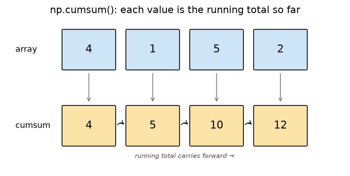
Because our prices are in weekly order, some NumPy functions are especially useful. np.cumsum() gives the cumulative sum: the running total spent after each week.
# Running total if you bought one gallon each week
np.cumsum(gas_prices)
array([ 3.047, 6.09 , 9.199, 12.302, 15.384, 18.512, 21.66 ,
24.785, 27.863, 30.932, 33.99 , 37.105, 40.267, 43.51 ,
46.678, 49.819, 52.952, 56.099, 59.219, 62.392, 65.552,
68.679, 71.787, 74.926, 78.139, 81.303, 84.428, 87.558,
90.679, 93.802, 96.942, 100.06 , 103.185, 106.332, 109.509,
112.701, 115.869, 119.042, 122.16 , 125.284, 128.345, 131.364,
134.399, 137.418, 140.474, 143.536, 146.597, 149.582, 152.522,
155.417, 158.258, 161.069])A small example shows the mechanics more clearly than 52 weeks of data. Each value in the running total is the sum of the corresponding array value and every value before it, so the running total carries forward from one box to the next:
Even more useful for a time series is np.diff(), which gives the difference between each value and the one before it: how much the price changed from one week to the next.
# Week-to-week changes in the price of gas
weekly_changes = np.diff(gas_prices)
weekly_changes
array([-0.004, 0.066, -0.006, -0.021, 0.046, 0.02 , -0.023, -0.047,
-0.009, -0.011, 0.057, 0.047, 0.081, -0.075, -0.027, -0.008,
0.014, -0.027, 0.053, -0.013, -0.033, -0.019, 0.031, 0.074,
-0.049, -0.039, 0.005, -0.009, 0.002, 0.017, -0.022, 0.007,
0.022, 0.03 , 0.015, -0.024, 0.005, -0.055, 0.006, -0.063,
-0.042, 0.016, -0.016, 0.037, 0.006, -0.001, -0.076, -0.045,
-0.045, -0.054, -0.03 ])np.diff() works on the same example: each output value is the difference between two adjacent inputs, so there is one fewer output than input:
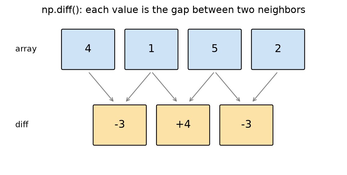
The result has 51 values rather than 52, because 52 weeks produce only 51 gaps. Now we can answer an interesting question: what was the single largest weekly change in price? Since a change can be a drop (negative) or a rise (positive), we use np.abs() to look at the size of each change regardless of direction, and np.max() to find the biggest:
# The size of the largest single-week change
np.max(np.abs(weekly_changes))np.float64(0.08099999999999996)The biggest swing in any week was about 8 cents. Combining this with np.argmax() and our dates, we can find exactly which week saw that change. There is one subtlety: because weekly_changes describes the gaps between weeks, its positions are shifted by one from the weeks themselves. The first change (position 0) is the jump from week 0 to week 1, so it belongs to week 1; the change at any position therefore corresponds to the date one position later. That’s why we add 1 before looking up the date:
# The week in which the largest change occurred.
# We add 1 because each change belongs to the *later* of the two weeks it spans.
gas_dates[np.argmax(np.abs(weekly_changes)) + 1]np.datetime64('2025-04-07T00:00:00.000000')The line plot at the start of the chapter showed when prices moved. A histogram of weekly_changes shows how much prices typically moved from one week to the next:
plt.hist(weekly_changes, bins=15, edgecolor='black')
plt.xlabel("Week-to-week price change ($)")
plt.ylabel("Number of weeks")
plt.title("Distribution of weekly gas price changes, 2025")
plt.show()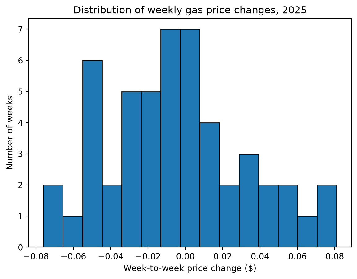
The changes cluster around zero: in most weeks the price moved less than five cents in either direction, and no week moved more than about eight cents.
TipExercise
Use np.diff() and np.min() to find the largest single-week drop in the price of gas (the most negative weekly change). Then find the date of the week in which it occurred.
NoteSolution
weekly_changes = np.diff(gas_prices)

# The largest drop is the most negative change, so we use np.min
largest_drop = np.min(weekly_changes)

# np.argmin gives the position of that drop; add 1 to get the later week
drop_date = gas_dates[np.argmin(weekly_changes) + 1]

[largest_drop, drop_date]
[np.float64(-0.07600000000000007), np.datetime64('2025-12-01T00:00:00.000000')]The largest single-week drop was about 8 cents, in the week ending in early December.
4.6 Boolean arrays and Boolean indexing
So far our questions have been about all the prices together. Often, though, we want to focus on values that meet some condition, such as the weeks where gas was cheap. NumPy handles this with Boolean arrays.
A Boolean array is just an array of True/False values. We can build one by hand, the same way we build any other array:
np.array([True, False, True])array([ True, False, True])More often, though, we create one by writing a comparison against an array. NumPy compares every element and returns an array of the results:
# Was the price below $3.00 in each week?
gas_prices < 3.00
array([False, False, False, False, False, False, False, False, False,
False, False, False, False, False, False, False, False, False,
False, False, False, False, False, False, False, False, False,
False, False, False, False, False, False, False, False, False,
False, False, False, False, False, False, False, False, False,
False, False, True, True, True, True, True])Because Python treats True as 1 and False as 0, we can count how many weeks met our condition by summing the Boolean array, and find the proportion of weeks by taking its mean:
# How many weeks was gas below $3.00?
np.sum(gas_prices < 3.00)np.int64(5)# What fraction of weeks was gas below $3.00?
np.mean(gas_prices < 3.00)np.float64(0.09615384615384616)Gas dipped below $3.00 in only 5 of the 52 weeks, or about 10% of the year. We can build more specific conditions by combining comparisons with & (“and”) and | (“or”). Each comparison must be wrapped in parentheses:
# How many weeks was the price between $3.00 and $3.20?
np.sum((gas_prices > 3.00) & (gas_prices < 3.20))np.int64(45)4.6.1 Boolean indexing
Beyond counting, we can use a Boolean array to pull out the values that meet a condition. This is called Boolean indexing or masking. To see how it works, start with a mask built by hand. Indexing an array with a Boolean array of the same length keeps the values where the mask is True and drops the values where it is False:
small_prices = np.array([3.05, 3.04, 3.11])
mask = np.array([True, False, True])

small_prices[mask]
array([3.05, 3.11])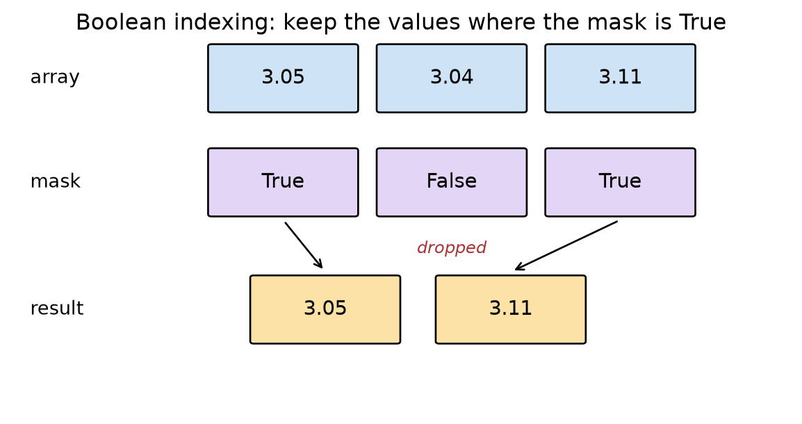
In practice we rarely type a mask by hand. Instead we produce one with a comparison, then index with it in a single expression:
# The actual prices for the weeks when gas was below $3.00
gas_prices[gas_prices < 3.00]
array([2.985, 2.94 , 2.895, 2.841, 2.811])The full value of masking appears when you then summarize the selected values. For example, among the weeks when gas was below $3.00, what was the average price?
np.mean(gas_prices[gas_prices < 3.00])np.float64(2.8944)Masking also lets us fulfill a promise from the previous chapter: finding a dataset’s outliers. Recall the rule of thumb that flags any value more than 1.5 IQRs below the 25th percentile or above the 75th percentile. With np.percentile() and a compound condition, this takes only a few lines:
q1 = np.percentile(gas_prices, 25)
q3 = np.percentile(gas_prices, 75)
iqr = q3 - q1

lower_fence = q1 - 1.5 * iqr
upper_fence = q3 + 1.5 * iqr

# The prices that fall outside the fences
gas_prices[(gas_prices < lower_fence) | (gas_prices > upper_fence)]
array([2.895, 2.841, 2.811])The three outliers are the unusually cheap weeks at the very end of December, the same low tail we saw in the line plot.
4.6.2 The same idea on other data
The Bechdel Test data from the previous chapter gives a different example of the same idea. Recall that each movie either passes ("PASS") or fails ("FAIL") the test. The cell below loads the movies’ pass/fail status and international gross earnings into two arrays, again using the pandas loading code you can treat as a black box for now:
# Load the Bechdel data and pull two columns out as arrays
movies = pd.read_csv("https://raw.githubusercontent.com/fivethirtyeight/data/refs/heads/master/bechdel/movies.csv")
movies = movies[["binary", "intgross_2013$"]].dropna()

bechdel_status = movies["binary"].values
intl_gross = movies["intgross_2013$"].values
Using exactly the masking technique we just learned, we can compare the average earnings of movies that passed the test against those that failed:
# Average international gross for movies that PASS vs. FAIL the Bechdel Test
[np.mean(intl_gross[bechdel_status == "PASS"]),
 np.mean(intl_gross[bechdel_status == "FAIL"])]
[np.float64(167359970.8358396), np.float64(222529817.73807105)]Movies that failed the Bechdel Test earned more on average than those that passed, the pattern FiveThirtyEight highlighted in its original analysis. The masking syntax is identical to the gas-price examples above. (Note that bechdel_status is an array of strings, like the mixed-type example earlier in the chapter, and comparisons work on it the same way they work on numbers.)
TipExercise
Using the gas_prices array, count how many weeks the price was above the average price for the year. (Hint: you can use np.mean(gas_prices) directly inside a comparison.)
NoteSolution
np.sum(gas_prices > np.mean(gas_prices))np.int64(34)The price was above the yearly average in 34 of the 52 weeks. (More than half the weeks can sit above the mean because the unusually cheap weeks at the end of the year pull the mean down, below the median.)
4.7 Higher-dimensional arrays and image processing
Every array we’ve used so far has been one-dimensional: a single row of numbers. But arrays can have more than one dimension. A two-dimensional array is just a grid of numbers, with rows and columns like a spreadsheet.
4.7.1 Creating and indexing matrices
A matrix is a 2D array, and the most direct way to build one is to pass np.array() a list of lists, with each inner list becoming one row:
matrix = np.array([
    [1, 2, 3],
    [4, 5, 6],
])

matrix
array([[1, 2, 3],
[4, 5, 6]])The .shape confirms the structure: 2 rows and 3 columns.
matrix.shape(2, 3)Indexing a 2D array takes two positions separated by a comma: a row, then a column. matrix[0, 1] is the value in row 0, column 1:
matrix[0, 1]np.int64(2)A : in either position means “every value along that axis.” matrix[1, :] pulls out all of row 1, and matrix[:, 2] pulls out all of column 2:
[matrix[1, :], matrix[:, 2]][array([4, 5, 6]), array([3, 6])]Slicing combines with indexing the same way: matrix[0:2, 1:3] keeps rows 0 and 1, and within those rows, columns 1 and 2:
matrix[0:2, 1:3]array([[2, 3],
[5, 6]])The axis argument in NumPy functions specifies which dimension to operate along. On a 2D array, axis=0 operates down the rows, producing one result per column, and axis=1 operates across the columns, producing one result per row:
# Sum down the rows (axis=0): one total per column
np.sum(matrix, axis=0)
array([5, 7, 9])# Sum across the columns (axis=1): one total per row
np.sum(matrix, axis=1)array([ 6, 15])The picture below shows the direction each version sums along, and the 1D array each one produces:
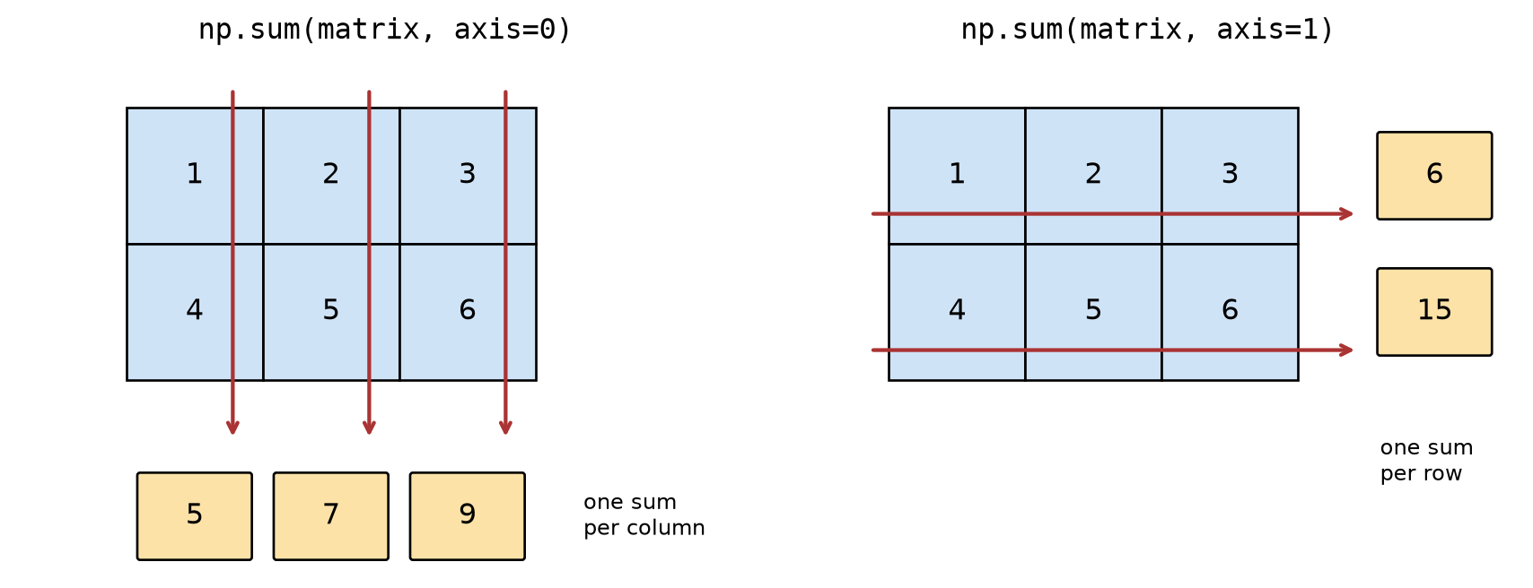
We will use this same idea with axis=2 when working with 3D color images later in this section.
TipExercise
Create the matrix [[1, 2, 3], [4, 5, 6], [7, 8, 9]] using np.array(). Then use indexing to pull out the value 7, and slicing to pull out the entire bottom row.
NoteSolution
small_matrix = np.array([
    [1, 2, 3],
    [4, 5, 6],
    [7, 8, 9],
])

[small_matrix[2, 0], small_matrix[2, :]]
[np.int64(7), array([7, 8, 9])]4.7.2 Grayscale images are 2D arrays
For a large grid, typing out every value as a list of lists is impractical, so we can ask NumPy to build the array for us. Here we start with a 100×100 grid of zeros using np.zeros(), then use slicing to set a square block of values in the middle to 1. Note that the [100, 100] we pass to np.zeros() is not a list of values (the way np.array([3.05, 3.04]) was). It describes the shape we want: 100 rows and 100 columns. NumPy functions that accept a shape always expect it as a single list or tuple, not as separate arguments.
# A 100x100 grid of zeros (100 rows, 100 columns)
grid = np.zeros([100, 100])

# Set a square block of the grid to 1 using slicing on both dimensions
grid[30:70, 30:70] = 1
Why make a grid of numbers? Because a grayscale image is exactly that: a 2D array where each number is the brightness of a pixel. If we display our grid as an image, the 1s show up as a white square on a black background:
plt.imshow(grid, cmap="gray")
plt.show()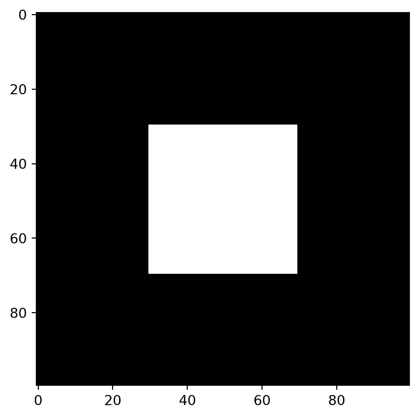
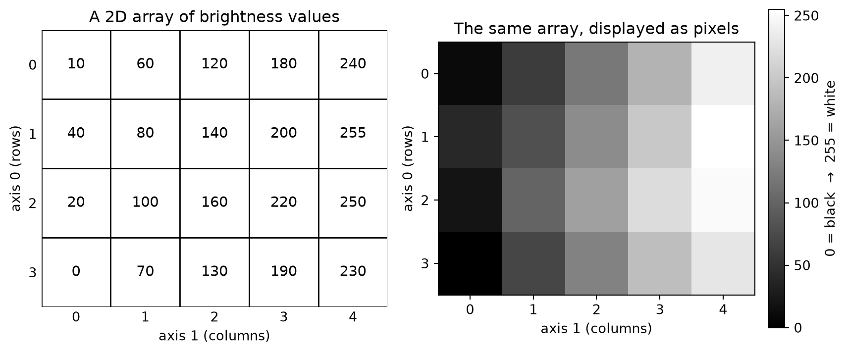
The picture below makes the connection precise: every position in the array has a row index (axis 0) and a column index (axis 1), and the value stored at that position controls how dark or light the pixel is. Stored photos typically use whole numbers from 0 (black) to 255 (white). (Our square example used 0 and 1 instead; by default Matplotlib stretches an array’s smallest value to black and its largest to white, which is why the 1s displayed as pure white.)
As a concrete example, consider the cameraman: a standard grayscale test image distributed with the imageio package and used in image-processing research for decades. Unlike most digital photos, it was stored from the start as a single 2D layer of brightness values with no color information:
from imageio.v3 import imread  # imread loads an image file into a NumPy array

# The "imageio:" prefix refers to a sample image bundled with the imageio
# package, not a file on your computer
cameraman = imread("imageio:camera.png")

plt.imshow(cameraman, cmap="gray")
plt.show()
Imageio: 'camera.png' was not found on your computer; downloading it now.
Try 1. Download from https://github.com/imageio/imageio-binaries/raw/master/images/camera.png (136 kB)
Downloading: 8192/139512 bytes (5.9%)139512/139512 bytes (100.0%)
Done
File saved as /home/runner/.imageio/images/camera.png.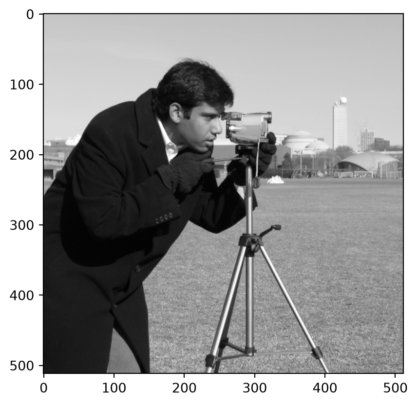
Confirm that it really is a 2D array of numbers by checking its shape and data type:
[cameraman.shape, cameraman.dtype][(512, 512), dtype('uint8')]The shape (512, 512) tells us the photo is 512 pixels tall and 512 pixels wide, with a single brightness value at each position, just like the small example above. The data type uint8 is an unsigned 8-bit integer: u means no negative values, and 8 bits gives exactly 256 possible values, from 0 to 255. Here 0 is black and 255 is white.
4.7.3 Color images are 3D arrays
Color photographs add a third dimension. Here we load a photo of bell peppers:
# Load the image into a NumPy array (same imread as above; the file is stored locally)
peppers = imread("images/peppers.jpg")

plt.imshow(peppers)
plt.show()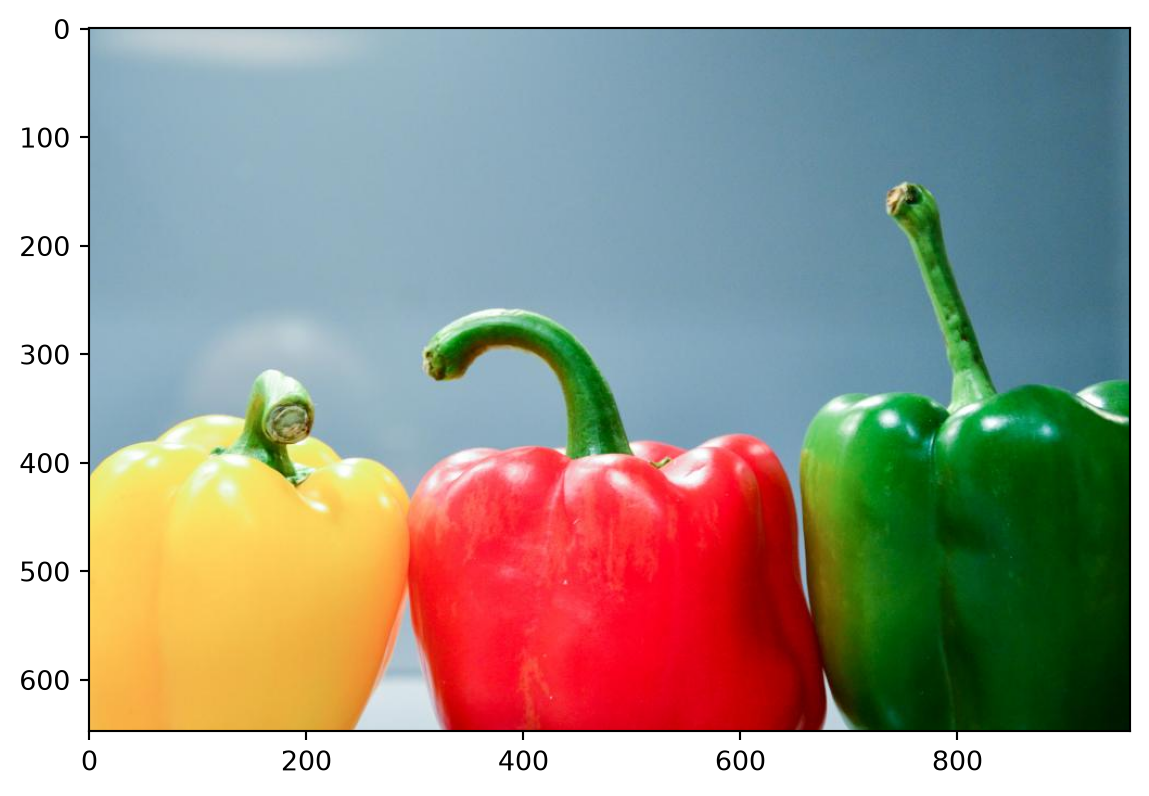
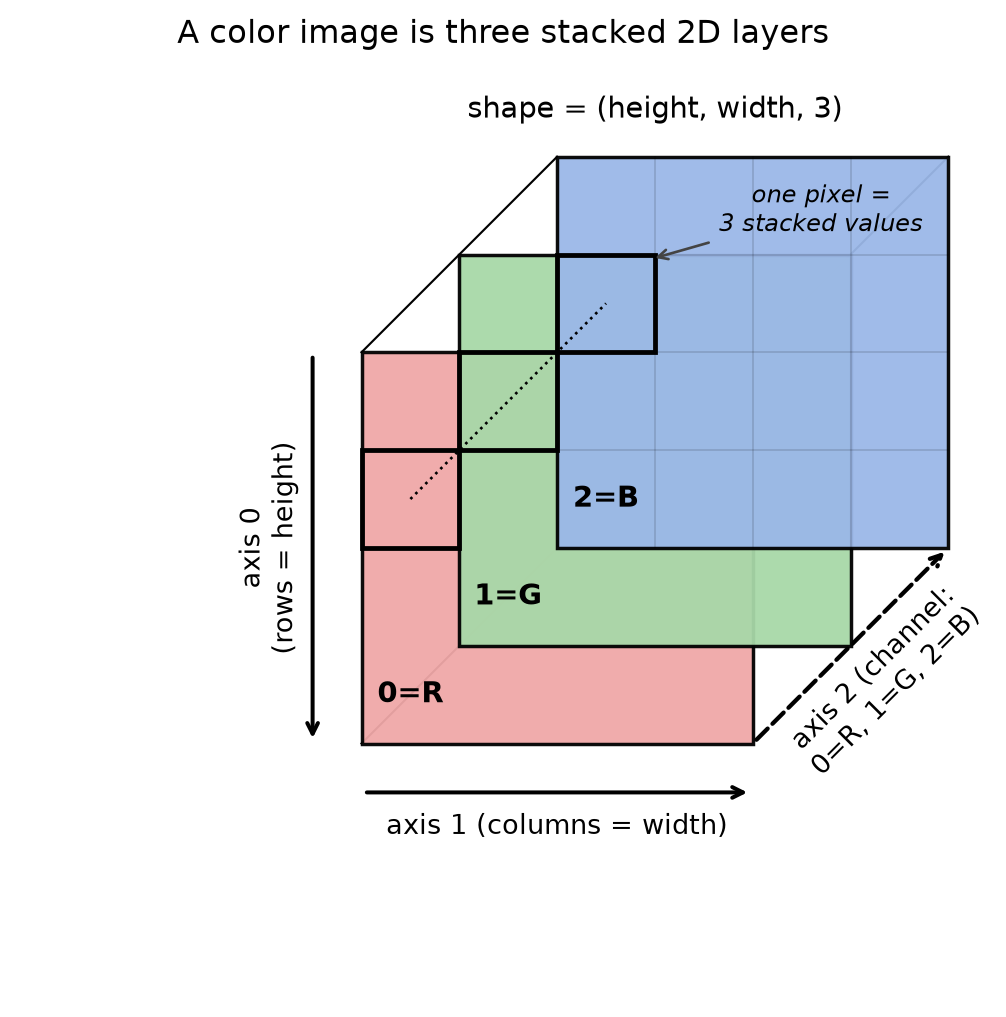
[peppers.shape, peppers.dtype][(648, 960, 3), dtype('uint8')]The shape (648, 960, 3) says the image is 648 pixels tall and 960 pixels wide, with 3 values at each pixel position, one per color channel. Each channel holds the intensity of one color (red, green, or blue) at that pixel, using the same uint8 range of 0 to 255. The diagram below shows how those three layers are organized; the outlined cell marks a single pixel, whose color is stored as three values at the same (row, column) position, one on each layer.
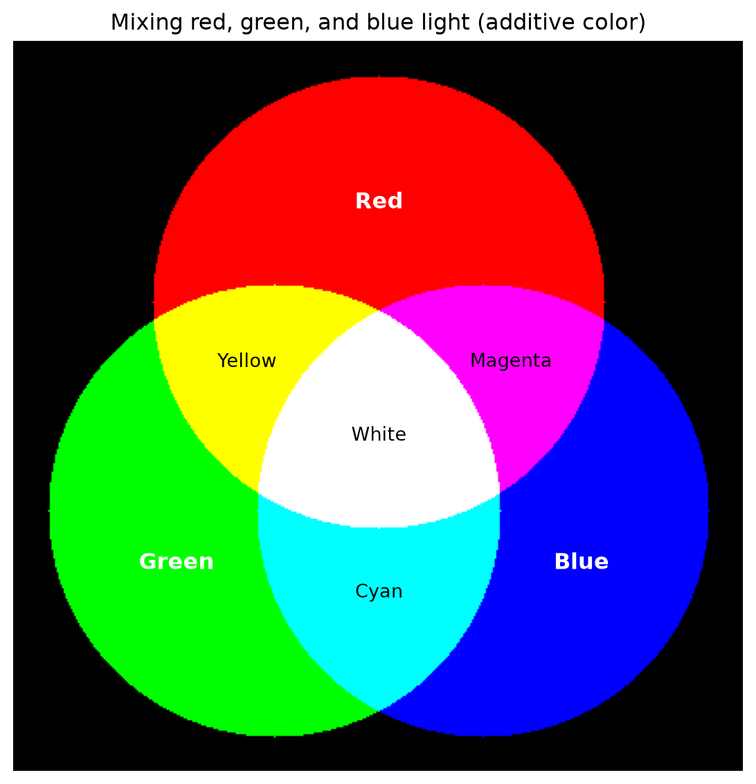
Combining different amounts of red, green, and blue light is how each pixel’s color is produced, an idea called additive color. Mixing any two of the three at full intensity produces yellow, magenta, or cyan; mixing all three produces white:
Averaging the red, green, and blue values at each pixel collapses them to a single brightness value, in the same format as the grayscale photo earlier. Passing axis=2 to np.mean() tells NumPy to average along the channel dimension: for each pixel position (row, column), it reduces the three channel values to one number, leaving an array of shape (height, width):
# Average the red, green, and blue values at each pixel
gray_peppers = np.mean(peppers, axis=2)

plt.imshow(gray_peppers, cmap="gray")
plt.show()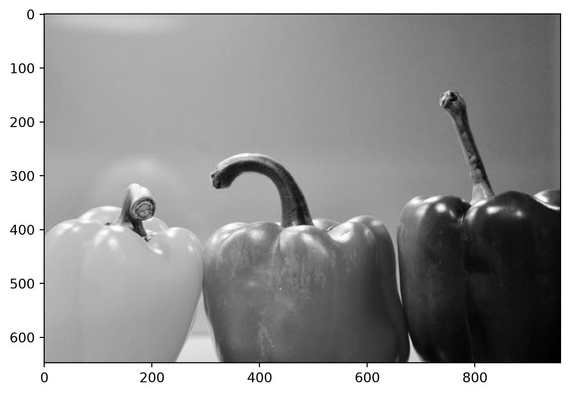
4.7.4 Manipulating an image is just array computation
Because the image is an array, every NumPy tool from this chapter applies to it. Using slicing, we can pull out a single color channel (here, the red channel) and display it on its own. The effect is visible across the peppers: the red one appears nearly white (high red-channel values), while the green one appears dark (low red-channel values). The yellow pepper also appears bright, and the additive-color figure explains why: yellow is red plus green light, so its red channel is high too:
# Keep all rows and columns, but only the first (red) channel
red_channel = peppers[:, :, 0]

plt.imshow(red_channel, cmap="gray")
plt.show()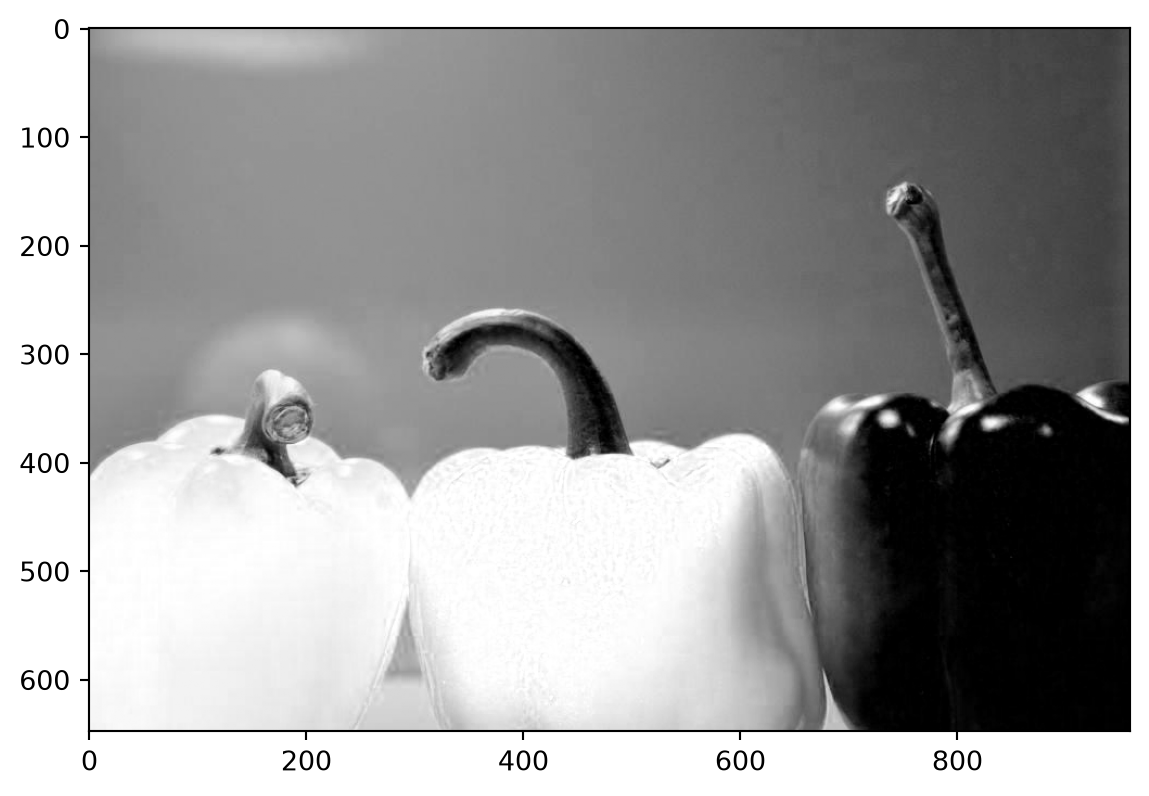
The Boolean-array idea works on images too. Comparing the grayscale image to a threshold produces a Boolean array marking the brightest pixels, which we can display to highlight the lightest regions of the photo:
# A Boolean array that is True for bright pixels
bright_pixels = gray_peppers > 150

plt.imshow(bright_pixels, cmap="gray")
plt.show()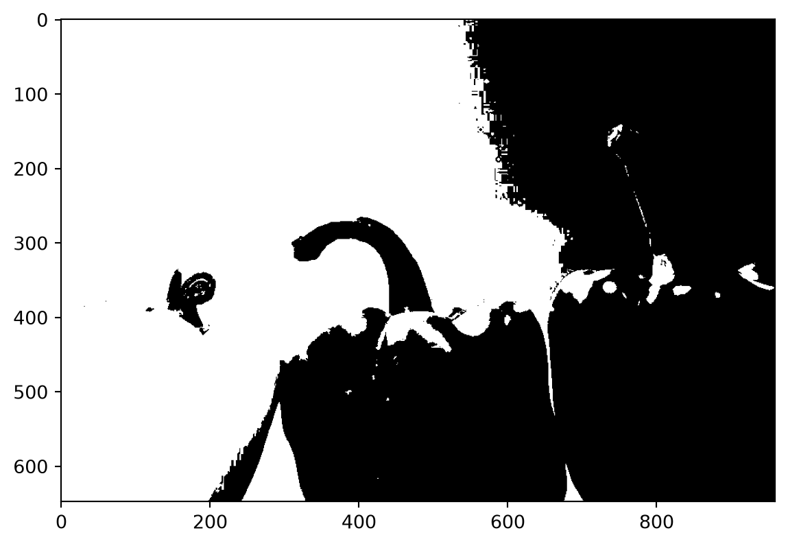
The white regions are the pixels where the condition was True: here, the bright sky in the background and the yellow pepper.
Images are just arrays. Slicing, arithmetic, np.mean() with an axis argument, and Boolean masks all work on image arrays the same way they work on any NumPy array.
TipExercise
Using the gray_peppers array from above, use Boolean indexing to count how many of its pixels are darker than a brightness of 50.
NoteSolution
# Count the pixels whose brightness is below 50
np.sum(gray_peppers < 50)np.int64(80398)4.8 Summary
In this chapter we introduced NumPy arrays, the standard container for numerical data in Python. The key ideas were:
- Arrays vs. lists. Arrays hold values of a single type and support vectorized operations, letting us transform every element at once instead of writing loops. This makes code shorter to write and faster to run.
- Creating and inspecting arrays. We build arrays with
np.array(),np.arange(), andnp.linspace(), and inspect them with attributes like.shape,.dtype,.size, and.ndim. - Summarizing and transforming. Functions such as
np.mean(),np.median(),np.min(),np.max(),np.sum(),np.std(), andnp.percentile()reduce an array to a single number, whilenp.diff()andnp.cumsum()are especially useful for sequences like time series. - Boolean arrays. Comparisons produce arrays of
True/Falsevalues that we can sum to count, average to find proportions, and use to index, pulling out and summarizing exactly the values that meet a condition. - Higher-dimensional arrays. Two- and three-dimensional arrays represent grids and images, and every array tool we learned applies to them.
Nearly every data science tool in Python builds on NumPy. In the chapters ahead we’ll use it to work with full data tables and to create richer visualizations.
4.9 Code summary
The functions and methods introduced in this chapter. NumPy is imported as np.
Creating arrays
| Code | What it does |
|---|---|
np.array([1, 2, 3]) |
Builds an array from a list |
np.arange(start, stop) |
Whole numbers from start up to but not including stop |
np.linspace(start, stop, n) |
n evenly spaced values, including both endpoints |
np.zeros(shape) |
An array of the given shape filled with zeros |
arr.astype(float) |
A copy of the array converted to another type |
arr.copy() |
An independent copy, so changing one does not change the other |
What an array is made of
| Code | What it does |
|---|---|
arr.shape |
The size along each dimension, as a tuple |
arr.size, arr.ndim |
How many values in total, and how many dimensions |
arr.dtype |
The kind of value the array holds |
Computing on every value at once
| Code | What it does |
|---|---|
arr + 1, arr * 2 |
Arithmetic applied to every value, without a loop |
np.abs(arr) |
The distance of each value from zero |
np.cumsum(arr) |
A running total, one value per position |
np.diff(arr) |
The gap between each pair of neighbors, giving one fewer value |
Summarizing an array
| Code | What it does |
|---|---|
np.mean(arr), np.median(arr) |
The average and the middle value |
np.std(arr) |
The standard deviation |
np.sum(arr) |
The total |
np.min(arr), np.max(arr) |
The smallest and largest value |
np.argmin(arr), np.argmax(arr) |
The position of the smallest or largest value |
np.percentile(arr, p) |
The value below which p percent of the data falls |
Selecting values
| Code | What it does |
|---|---|
arr[0], arr[-1] |
One value, by position, counting from zero |
arr[1:4] |
A slice, from position 1 up to but not including 4 |
arr > 3 |
An array of True and False, one per value |
arr[arr > 3] |
Keeps only the values where the condition is True |
(arr > 1) & (arr < 4) |
Combines conditions, with & for and and | for or |
np.sum(mask), np.mean(mask) |
Counts how many are True, and what fraction are |
Two- and three-dimensional arrays
| Code | What it does |
|---|---|
matrix[row, col] |
One value, by row and column |
matrix[0:2, 0:2] |
A rectangular block of the array |
np.sum(matrix, axis=0) |
Summarizes down the columns; axis=1 works across the rows |
imread("file.jpg") |
Reads an image into an array of pixel values |
plt.imshow(img) |
Displays an array as a picture |
4.10 Exercises
TipExercise
Create a NumPy array of the gas prices expressed in cents rather than dollars (so $3.05 becomes 305 cents). Then find the average price in cents.
NoteSolution
prices_in_cents = gas_prices * 100

[prices_in_cents, np.mean(prices_in_cents)]
[array([304.7, 304.3, 310.9, 310.3, 308.2, 312.8, 314.8, 312.5, 307.8,
306.9, 305.8, 311.5, 316.2, 324.3, 316.8, 314.1, 313.3, 314.7,
312. , 317.3, 316. , 312.7, 310.8, 313.9, 321.3, 316.4, 312.5,
313. , 312.1, 312.3, 314. , 311.8, 312.5, 314.7, 317.7, 319.2,
316.8, 317.3, 311.8, 312.4, 306.1, 301.9, 303.5, 301.9, 305.6,
306.2, 306.1, 298.5, 294. , 289.5, 284.1, 281.1]),
np.float64(309.74807692307695)]
TipExercise
The range of a dataset is the difference between its largest and smallest values. Use np.max() and np.min() to compute the range of the gas prices for the year.
NoteSolution
np.max(gas_prices) - np.min(gas_prices)np.float64(0.43199999999999994)Gas prices varied by about 43 cents between the cheapest and most expensive weeks of the year.
TipExercise
Use slicing and np.mean() to compare the average gas price in the first half of the year (the first 26 weeks) to the average in the second half (the last 26 weeks). Did gas get cheaper or more expensive on average?
NoteSolution
first_half_avg = np.mean(gas_prices[0:26])
second_half_avg = np.mean(gas_prices[26:52])

[first_half_avg, second_half_avg]
[np.float64(3.127038461538461), np.float64(3.0679230769230768)]Gas was more expensive in the first half of the year than in the second half, consistent with the downward drift we saw in the line plot.
TipExercise
In this chapter we compared movies that passed and failed the Bechdel Test using only their average international gross. Averages can hide a lot. Use Boolean masking to create two arrays, pass_gross and fail_gross, holding the international gross of the passing and failing movies. Then display them as side-by-side box plots (which you met in the previous chapter) by passing a list of the two arrays to plt.boxplot(). Does the comparison look different from the comparison of means?
NoteSolution
pass_gross = intl_gross[bechdel_status == "PASS"]
fail_gross = intl_gross[bechdel_status == "FAIL"]

plt.boxplot([pass_gross, fail_gross])
plt.xticks([1, 2], ["PASS", "FAIL"])
plt.ylabel("International gross (2013 dollars)")
plt.title("International gross by Bechdel Test result")
plt.show()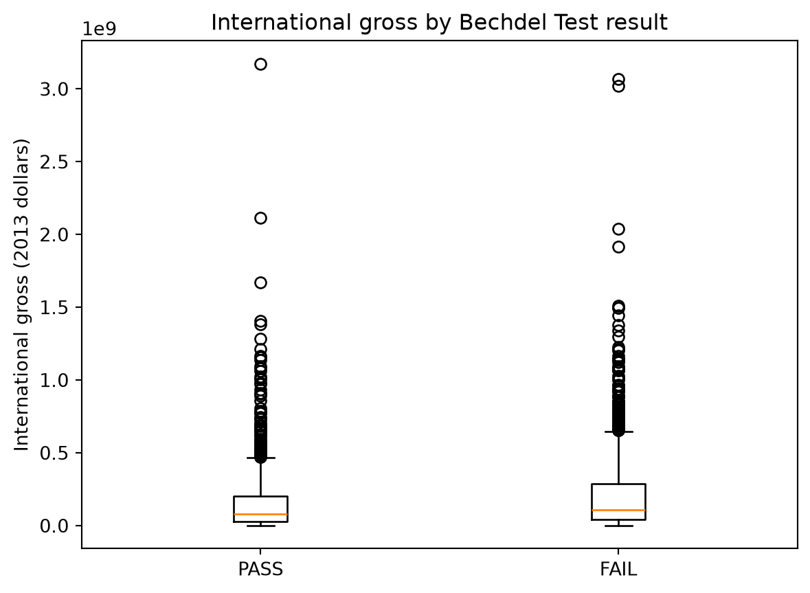
The two distributions overlap heavily, and both are dominated by a small number of very high-grossing outlier movies. The difference between the groups looks much less dramatic here than the comparison of means suggested, a reminder that a single summary number can hide the shape of the data.
TipExercise
Create a version of the peppers image with the red and blue channels swapped, and display it. (Hint: make a copy first with swapped = peppers.copy() so you don’t change the original, then use slice assignment to set the copy’s red channel to the original’s blue channel and vice versa.)
NoteSolution
swapped = peppers.copy()

# Set the copy's red channel to the original's blue channel, and vice versa
swapped[:, :, 0] = peppers[:, :, 2]
swapped[:, :, 2] = peppers[:, :, 0]

plt.imshow(swapped)
plt.show()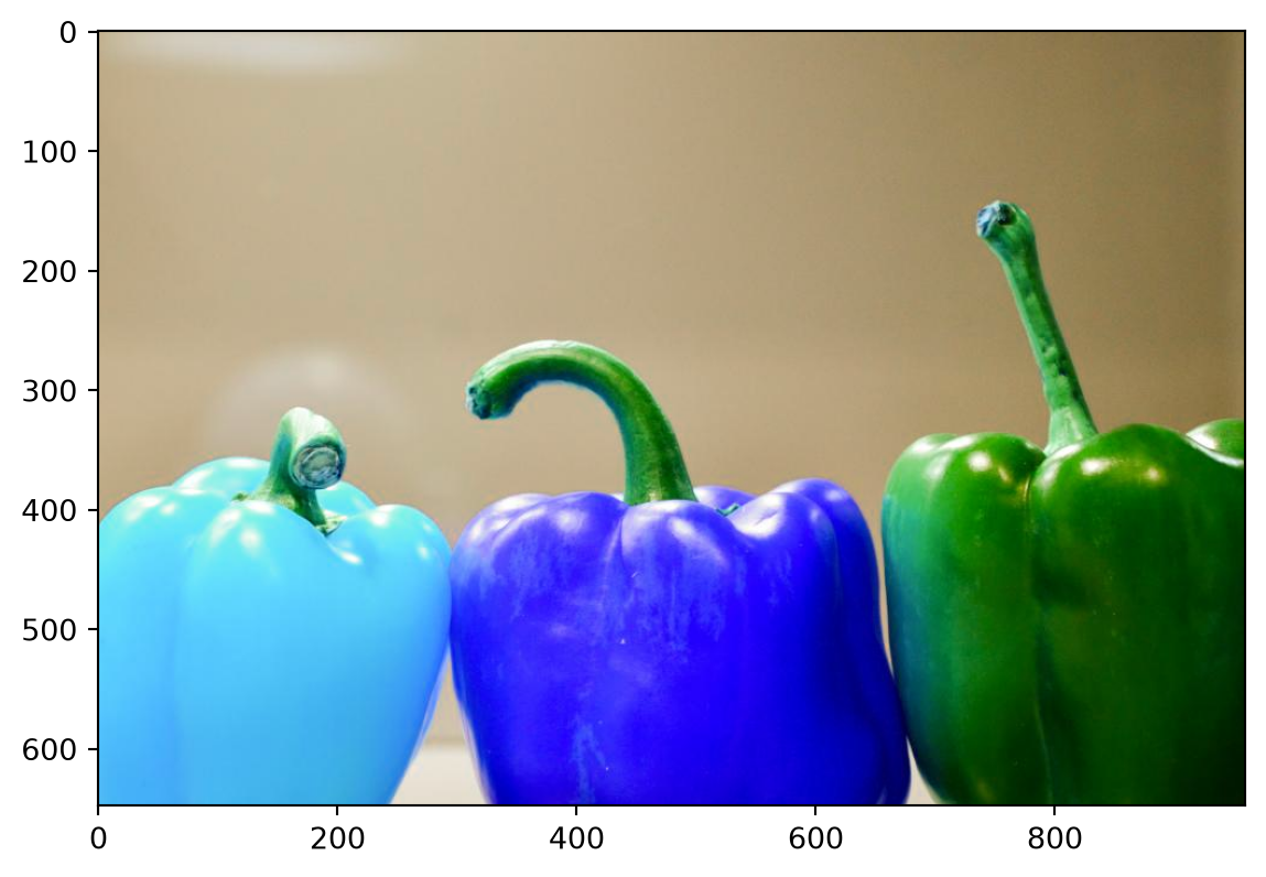
The red pepper now appears blue and the yellow pepper turns cyan (its red light became blue light, and cyan is green plus blue). The green pepper barely changes, since its color lives mostly in the untouched green channel.